A ground-up tutorial on the architecture of Large Language Models (LLMs) and Large Multimodal Models (LMMs) — explained the way you’d want it explained if you were going to build with them.
Table of Contents
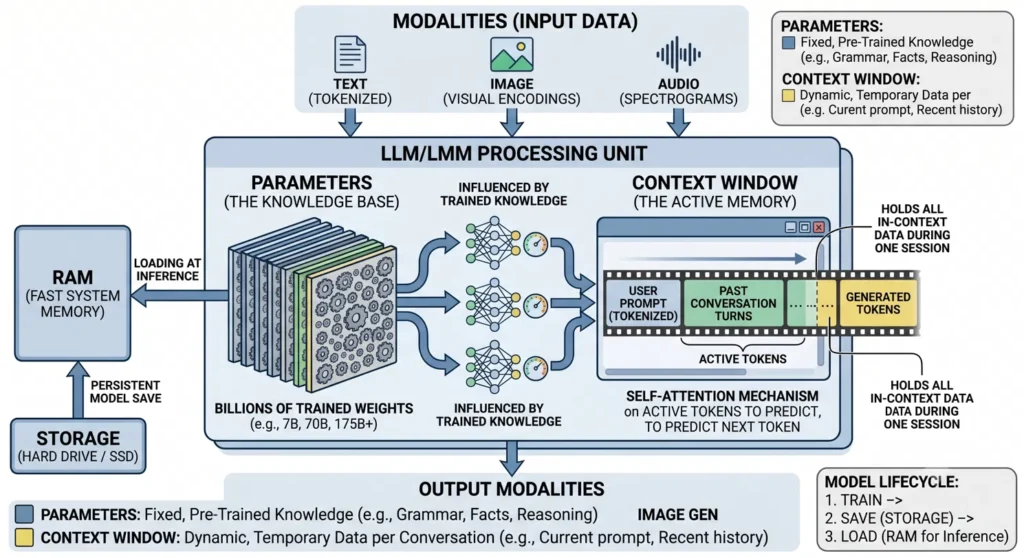
The one-sentence mental model
An LLM is a giant fixed function that takes a sequence of tokens and outputs a probability distribution for the next token. Everything else — chat, reasoning, code generation — is that single trick run in a loop.
Hold onto that. Every concept below is just a piece of that sentence. There are two things you must keep separate in your head, because confusing them is the #1 source of mistakes:
| Parameters | Context Window | |
|---|---|---|
| What it is | The model’s baked-in knowledge | The model’s working memory for this conversation |
| When it’s set | During training (then frozen) | Fresh every request |
| Analogy | Everything you learned in school | The notepad in front of you right now |
| Changes per chat? | No — identical for every user | Yes — unique to each prompt |
| Size | Fixed (e.g. 7B, 70B numbers) | Limited (e.g. 8k, 128k, 1M tokens) |
A model does not learn from your conversation. The parameters are read-only at inference time. Anything “remembered” lives in the context window and vanishes when the window closes. Keep this table in mind and 90% of LLM behavior stops being mysterious.
1. Tokens — the atoms of the model
LLMs don’t see letters or words. They see tokens: chunks of text mapped to integers.
A token is usually a piece of a word, not a whole word. The tokenizer splits text using a learned scheme (most models use Byte-Pair Encoding, BPE, or a variant like SentencePiece). Common words become a single token; rare words get split into pieces.
"tokenization"  ->  ["token", "ization"]      (2 tokens)
"The cat sat."  ->  ["The", " cat", " sat", "."]  (4 tokens)
"Chevilly"      ->  ["Che", "v", "illy"]       (3 tokens — rare word, more pieces)
Notice the space is usually glued to the front of the next token (" cat"). That’s not a bug — it’s how BPE keeps word boundaries.
Rules of thumb (English):
- ~1 token ≈ 4 characters
- ~1 token ≈ 0.75 words
- 100 tokens ≈ 75 words ≈ 1 short paragraph
Why this matters in practice:
- You pay per token, not per word. API pricing, rate limits, and context limits are all counted in tokens.
- Non-English and code cost more tokens. French accents, Tibetan script, JSON with lots of punctuation — all fragment into more tokens than plain English. A French paragraph can cost 20–40% more tokens than its English equivalent.
- The model’s “spelling weakness” (miscounting letters in a word) comes from this: it literally never sees the letters, only the token chunks.
Feynman check: Why can’t an LLM reliably count the R’s in “strawberry”? Because “strawberry” might be 2–3 tokens, and the model sees those as opaque IDs — it never sees the individual letters at all. It’s like being asked how many strokes are in a Chinese character you only know by its sound.
2. Vocabulary — the model’s fixed alphabet of tokens
The vocabulary is the complete, fixed list of every token the model knows. Each token has a unique ID:
"The"    -> 791
" cat"   -> 8415
" sat"   -> 7731
"."      -> 13
Modern vocabularies are large — typically 30,000 to 260,000 tokens:
| Model family | Approx. vocab size |
|---|---|
| Older GPT-2 era | ~50,000 |
| GPT-4 / cl100k tokenizer | ~100,000 |
| Llama 3 | ~128,000 |
| Gemini | ~256,000 |
Bigger vocabulary = fewer tokens per sentence (each token carries more meaning), but a bigger embedding table to store. It’s a trade-off the model designers fix once, before training.
The vocabulary is decided before training and never changes afterward. This is why a model can’t invent a brand-new token for a word it has never seen — it just splits the unknown word into known sub-pieces. Every input and every output is ultimately a sequence of these vocabulary IDs.
The full pipeline so far:
Your text  ->  [tokenizer]  ->  token IDs  ->  [MODEL]  ->  token IDs  ->  [detokenizer]  ->  text
"Bonjour"      splits into     [12, 4567]      magic       [9023, ...]     reassembles       "Hello"
3. Parameters (weights) — the knowledge base
Now the model itself. A parameter is a single number (a weight) learned during training. An LLM is nothing but billions of these numbers arranged in matrices, plus the simple arithmetic that multiplies your tokens through them.
When you read “7B”, “70B”, “175B” — that’s the parameter count. 7B = 7 billion numbers.
What’s actually stored in those numbers? Compressed statistical knowledge about language: grammar, facts, reasoning patterns, coding conventions, style. There is no database of sentences inside. The model “knows” the capital of France not because it stored that sentence, but because the weights encode a relationship that makes “Paris” the high-probability continuation of “The capital of France is”.
This is why parameters are the fixed, pre-trained knowledge in your diagram. They are:
- Frozen at inference — identical for every request, every user.
- The thing you download when you pull a model with Ollama or from Hugging Face. A
.ggufor.safetensorsfile is the parameters.
How big is a parameter on disk?
Each weight is a number stored at some precision:
| Precision | Bytes per parameter | Notes |
|---|---|---|
| FP32 (full) | 4 bytes | Training; rarely used for inference |
| FP16 / BF16 (half) | 2 bytes | Standard “full quality” inference |
| INT8 (8-bit quant) | ~1 byte | Light compression |
| INT4 (4-bit quant) | ~0.5 byte | Aggressive compression, very common locally |
So the file size is roughly parameter count × bytes per parameter:
7B model at FP16  = 7,000,000,000 × 2 bytes ≈ 14 GB
7B model at 4-bit = 7,000,000,000 × 0.5    ≈ 3.5 GB  (+ a little overhead)
70B model at 4-bit ≈ 35–40 GB
This is the single most useful formula for self-hosting. Want to know if a model fits on your box? Multiply params × bytes-per-param. That’s your baseline. (We’ll add the context-window cost next.)
Quantization is the trick that makes local LLMs practical: take FP16 weights and round them into 4-bit buckets. You lose a little accuracy and gain a ~4× reduction in size and memory. For most tasks the quality drop is small; for precise reasoning or code it’s more noticeable. This is exactly the lever you pull when deciding between self-hosting a quantized model on a CPU box versus calling a hosted FP16 endpoint.
4. The Context Window — the active (working) memory
The context window is the model’s short-term memory: the maximum number of tokens it can “look at” in a single forward pass. Everything the model considers — system prompt, conversation history, your current message, retrieved documents, and the tokens it has generated so far — must fit inside this window.
Typical sizes today: 8k, 32k, 128k, even 1M tokens.
What goes in the window, in order:
[ SYSTEM PROMPT ][ PAST CONVERSATION TURNS ][ YOUR CURRENT PROMPT ]
[ GENERATED TOKENS ... ]
└────────────────────────────────────────────────┘
 all of this must fit in the context limit
The mental trap to avoid: the model is stateless
Here is the thing the diagrams almost never make clear:
The model does not remember your previous messages. The application re-sends them every single time.
Each time you hit “send” in a chat, the client glues together the entire conversation history + your new message into one big token sequence and feeds the whole thing to the model fresh. The model has no memory between calls. “Continuity” is an illusion maintained by the app resending the transcript.
Consequences that trip people up:
- Long chats get expensive and slow — every turn re-processes the whole growing history.
- When you exceed the window, the oldest tokens get dropped (or summarized). That’s why a model “forgets” what you said an hour ago: it literally fell out of the window.
- “Memory” features (like persistent user memory across chats) are not the context window. They’re an external store that the app injects into the window as text when relevant.
What the context window costs in RAM: the KV cache
The context window isn’t free memory-wise. As the model processes tokens, it stores intermediate results for every token in something called the KV cache (key/value cache). This cache grows linearly with how many tokens are in the window.
Approx. KV cache size ≈ 2 × layers × hidden_size × tokens × bytes_per_valueThe practical takeaway without the algebra: a long context can eat as much memory as the model weights themselves. A 7B model might be 4 GB of weights but need several more GB if you fill a 32k+ context. When you size a self-hosted box, budget for weights + KV cache, not just weights.
5. Self-attention — how the model uses the window
Inside the processing unit, the mechanism that makes all this work is self-attention (the “Transformer” architecture).
The Feynman version: for each token, the model asks “which of the other tokens in my window matter for predicting what comes next, and how much?” It computes a weighted blend of all the tokens in context, letting “it” connect back to the right noun, or a closing bracket connect to its opener 500 tokens earlier.
That’s why context matters so much: attention is the only way information from your prompt reaches the prediction. A token outside the window simply doesn’t exist to the model.
The cost: classic attention scales quadratically with context length (double the tokens → ~4× the attention compute). That’s the deep reason long contexts are slow and why 1M-token windows are an engineering achievement, not a free setting.
6. Inference — running the model (the loop)
Inference = using a trained model to generate output (as opposed to training, which created the weights). It happens in two phases.
Phase 1 — Prefill: the entire input prompt is pushed through the network in one pass, building the KV cache. This is the “first token takes a moment” delay.
Phase 2 — Decode (autoregressive generation): the model generates one token at a time, in a loop:
1. Run the current sequence through the parameters.
2. Get a probability for every token in the vocabulary (the "logits").
3. Pick the next token (sampling — see below).
4. Append it to the sequence.
5. Go to step 1, now including the token you just made.
... repeat until a stop token or length limit.
This is what “autoregressive” means: each new token is conditioned on everything before it, including the model’s own previous outputs. The model writes one word, reads its own writing, then writes the next.
Sampling — how the next token gets chosen (step 3 above). The model gives probabilities; how you pick from them controls the output’s character:
- Temperature — low (≈0) = pick the most likely token, deterministic and “safe”; high (≈1+) = more random and creative.
- Top-p / Top-k — only sample from the most probable tokens, cutting off the long tail of nonsense.
This is also the source of the famous truth about LLMs: they predict plausible text, not true text. A “hallucination” is just the model confidently sampling a high-probability continuation that happens to be false. The mechanism is identical whether the output is right or wrong.
7. The memory hierarchy: Storage vs RAM vs VRAM
This is where your diagram’s lifecycle (Train → Save → Load) lives, and it’s worth getting exactly right because it determines what hardware you need.
The three tiers
STORAGE (SSD/HDD)  ──load──►  RAM / VRAM  ──compute──►  output
   slow, huge,                 fast, smaller,
   permanent                   temporary
1. Storage (SSD / hard drive) — permanent home. The model file (the parameters) lives here. It’s persistent — survives reboots. It’s slow to read from, so you only touch it once: at load time. This is where Ollama keeps your pulled models.
2. RAM or VRAM — the working stage. To run the model, the parameters must be loaded off storage into fast memory, because the math runs there. This is the “Load at inference” arrow in your diagram. Which fast memory depends on your hardware:
| You run on… | Parameters load into… | This is your situation when… |
|---|---|---|
| GPU | VRAM (GPU memory) | You have an Nvidia card / use a GPU endpoint |
| CPU | System RAM | You self-host on a CPU-only server (e.g. a Hetzner CX-class VPS) |
Correction to the simplified diagram: the diagram labels the fast-memory box “RAM,” which is correct for CPU inference — but on a GPU, the weights go into VRAM, not system RAM, and VRAM is the scarce resource everyone fights over. On a CPU box, system RAM is your ceiling and the CPU is your speed bottleneck (CPU inference is much slower than GPU). This distinction decides your whole deployment strategy.
3. Compute (CPU cores / GPU cores) — does the multiplication. Once weights are in fast memory, the processor runs the token math. GPUs win massively here because they do thousands of multiplications in parallel — exactly the operation a Transformer needs.
The Model Lifecycle (your diagram’s bottom-right box, expanded)
1. TRAIN   — run huge data through the network, adjust billions of weights.
             Costs millions of dollars and weeks. Done once, by the model maker.
2. SAVE    — write the finished weights to STORAGE as a file. (the .gguf / .safetensors)
3. LOAD    — copy that file from storage into RAM/VRAM. Happens every time you start the server.
4. INFER   — run prompts through the loaded weights, one token at a time. (Sections 4–6)
You, as someone running models, only ever do steps 3 and 4. Training is upstream of you.
Sizing your hardware — the practical checklist
To know if a model will run on a given box, add up:
Total fast memory needed ≈  (model weights)  +  (KV cache for your context)  +  overhead (~1–2 GB)

Example — 7B model, 4-bit, 8k context on a CPU box:
   weights:    ~4 GB
   KV cache:   ~1–2 GB
   overhead:   ~1 GB
   ──────────────────────
   TOTAL:      ~6–7 GB of system RAM, and expect modest tokens/sec on CPU
If that total exceeds your RAM/VRAM, the model either won’t load or will spill to slow storage (swap) and crawl. This calculation is exactly what you weigh when choosing self-host on a CPU VPS (cheap, private, slow, RAM-bound) vs. a hosted GPU inference endpoint (fast, pay-per-token, your data leaves your box). There’s no universally right answer — it’s a cost/latency/privacy trade-off you make per workload.
8. LMM — extending from text to multimodal
An LMM (Large Multimodal Model) is the same machine, with extra front doors. The core is still “predict the next token using parameters + context window.” The only change is that other modalities get converted into tokens (or token-like vectors) the model can attend to.
TEXT   ──tokenizer──────────►  ┐
IMAGE  ──vision encoder─────►  ├──►  [ same Transformer + context window ]  ──►  output
AUDIO  ──audio encoder──────►  ┘        (one shared "language" of vectors)
- Text → tokenized as usual.
- Image → a vision encoder chops it into patches and turns them into vectors (“visual tokens”). A 512×512 image might cost hundreds to a thousand+ tokens of your context window — images are not free.
- Audio → converted to a spectrogram, then encoded into vectors the same way.
The crucial insight: everything becomes a sequence of vectors in one shared space, and the same self-attention mechanism mixes them. The model can “look at” an image patch and a word in the same breath because, internally, they’re the same kind of object. Output can also be multimodal (text, or generated images) by reversing the process.
So an LMM isn’t a different architecture — it’s the LLM with translators bolted onto the input (and sometimes output) side.
9. Putting it all together
Walk one request end to end:
- You type a prompt (text, maybe an image). → Modalities / input
- The tokenizer (and any encoders) turn it into token IDs from the fixed vocabulary.
- Those tokens, plus the conversation history the app re-sends, fill the context window.
- The tokens flow through billions of frozen parameters, which were loaded from storage into RAM/VRAM at startup.
- Self-attention lets every token weigh every other token in the window.
- The model outputs a probability over the whole vocabulary; sampling picks the next token. → this is inference.
- That token is appended and the loop repeats autoregressively until done.
- The token IDs are detokenized back into text (or an image). → output
The parameters never changed. The context window held everything temporary and will be discarded. Next request starts the cycle again, fresh.
Glossary (quick reference)
| Term | One-line definition |
|---|---|
| Token | A chunk of text (usually a word-piece) mapped to an integer; the unit the model reads and writes. |
| Tokenizer | The component that splits text into tokens and back again (usually BPE / SentencePiece). |
| Vocabulary | The fixed, complete list of all tokens a model knows (≈30k–260k); set before training, never changes. |
| Parameter / weight | One learned number. Billions of them = the model’s frozen knowledge (“7B” = 7 billion). |
| Quantization | Storing weights at lower precision (e.g. 4-bit) to shrink size and memory, trading a little accuracy. |
| Context window | Max tokens the model can attend to at once (prompt + history + output). The working memory. |
| KV cache | Per-token intermediate data stored during generation; makes context window cost real memory. |
| Self-attention | The Transformer mechanism letting each token weigh every other token in the window. |
| Inference | Running a trained model to generate output (vs. training, which created the weights). |
| Autoregressive | Generating one token at a time, each conditioned on all previous tokens including its own outputs. |
| Sampling (temperature/top-p) | How the next token is chosen from the predicted probabilities; controls creativity vs. determinism. |
| Prefill / decode | Inference’s two phases: process the whole prompt once, then generate tokens one by one. |
| Storage | Slow, permanent disk where the model file lives (.gguf / .safetensors). |
| RAM / VRAM | Fast memory the weights load into to run — system RAM for CPU inference, VRAM for GPU. |
| LMM | Multimodal model: same architecture, with encoders that turn images/audio into tokens. |
Tutorial draft. The architecture concepts here are stable and vendor-neutral; specific numbers (vocab sizes, context limits, pricing) evolve, so verify current figures for any model you actually deploy.